本文起因是我师兄有篇文章用到了配对样本数据,投稿后审稿人要求使用条件logistic回归(conditional logistic regression analysis),找了一些资料发现没有比较好的教程,都是在spss中使用cox回归曲线救国实现的,于是就去学习了下条件logistic回归在R语言中的实现。
审稿人意见:Case-control study needs to be accounted by means of a conditional logistic regression analysis (instead of “normal” logistic regression). There was no hint in the text, so in order to avoid any biased OR/mean estimates from the models mentioned the authors are kindly asked to provide a bit more information on the methodological approach.
概念及实现方法
条件logistic回归是由Norman Breslow, Nicholas Day, Katherine Halvorsen, Ross L. Prentice和C. Sabai在1978年提出,是logistic回归的延伸,允许人们考虑到分层和匹配,通常用于具有特定条件或属性的病例受试者与没有该条件的n个对照受试者相匹配。
原理部分不多赘述,我们只要知道当涉及到以下场景,出现了配对样本时(无论是1:1,1:n),都需要考虑使用该统计学方法。
适用场景:
1、倾向性评分匹配后的分析
2、巢式病例对照研究
3、病例对照研究
实现方法:
有现成的R包函数可以使用,分别是‘Survival’包中的clogit()函数,及Epi包中的clogistic()函数实现,本文主要以clogit来阐述。
clogit函数
阅读说明文档,该函数是专门用于Conditional logistic regression分析,有趣的是它计算也是基于cox回归的似然比分析,那说明前文提到的使用SPSS的方法也是有道理的。
An object of class “clogit”, which is a wrapper for a “coxph” object.
#函数基本格式
clogit(formula, data, weights, subset, na.action,
 method=c("exact", "approximate", "efron", "breslow"),
 ...)
变量说明
| formula* | Model formula |
|---|---|
| data* | data frame |
| weights | optional, names the variable containing case weights |
| subset | optional, subset the data |
| na.action | optional na.action argument. By default the global option na.action is used |
| method | use the correct (exact) calculation in the conditional likelihood or one of the approximations |
R语言实战
代码
没有采用示例中的数据,我们导入survival包内自带的数据集lung (NCCTG Lung Cancer Data)
rm(list = ls())  #清空一下工作空间
library(survival)
data_lung<-survival::lung
## 加入我自己定的结局变量和分组信息
outcome<- ifelse(data_lung$time <180,1,0)  #这里我们把180天内死亡设置为结局
id<-rep(1:76,3)   #假装是1:2对照,生成1:76三次
#id<-rep(1:76, each = 3) #生成比较连续的数字
data_lung$outcome<-outcome
data_lung$id<-id
#data_lung$outcome<-factor(data_lung$outcome) #这里千万不能将结局变量转化为因子,否则会运行报错
clogit_full<-clogit(outcome ~ sex + strata(id),data =  data_lung)  #以性别为单变量做回归,strata(id)为输入配对编号的位置
summary(clogit_full)
接着我们再用glm函数做一下性别的单因素Logistic回归
logistic_full<-glm(outcome ~ sex,data=data_lung,family = "binomial")
summary(logistic_full)
# 这里有个不好,glm函数的OR以及95%区间需要单独计算
exp(coef(logistic_full)) 计算OR值
exp(confint(logistic_full)) 计算95%区间
结果输出
结果1~条件Logistic回归
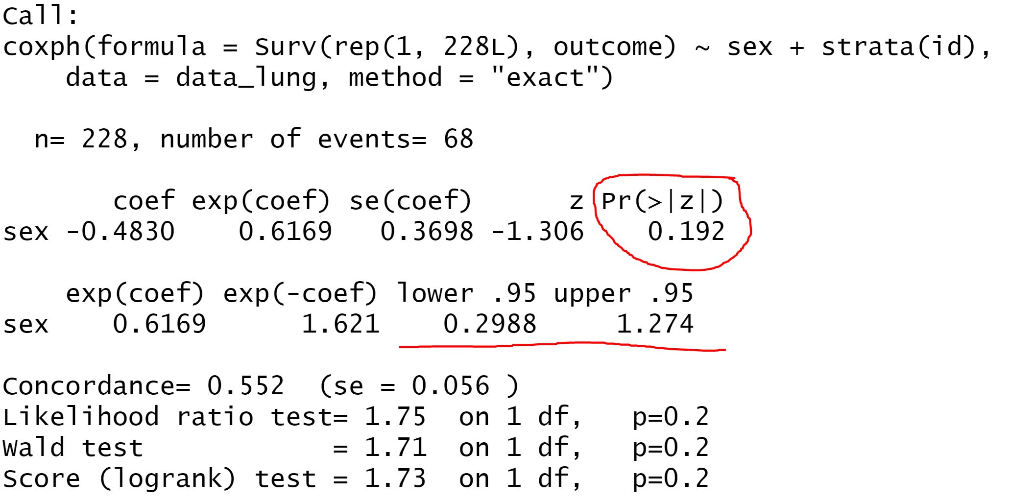
通过条件Logistic回归计算得出 0.617(0.299,1.274) p=0.192
结果2~Logistic回归
# 输出OR以及95%置信区间
                2.5 %    97.5 %
(Intercept) 0.4778247 2.6897932
sex         0.2582867 0.8875878
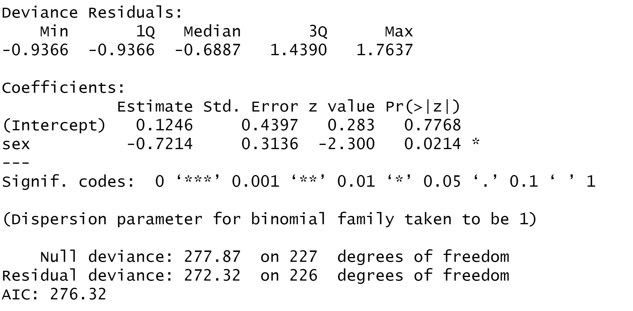
如果不考虑到配对因素去回归得出0.486(0.258,0.887) p=0.0214 *
结果3~SPSS中的条件Logistic回归
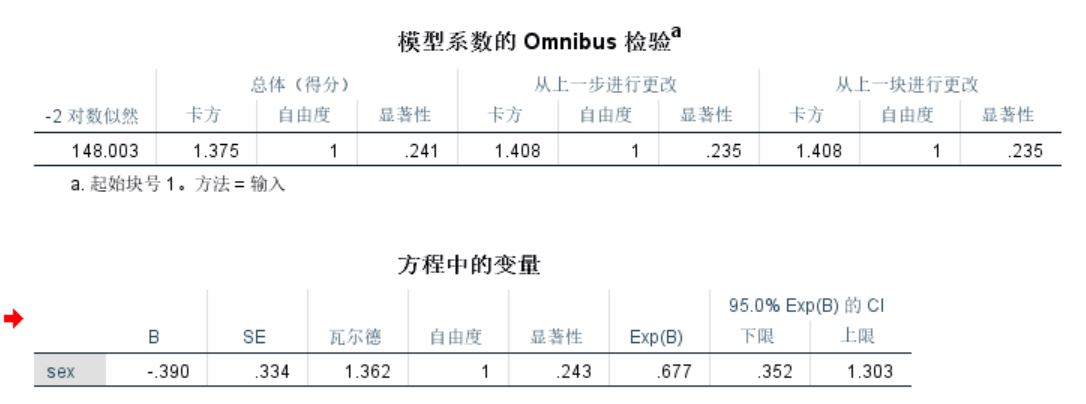
我也在SPSS中计算了一下,具体方法见条件Logistic回归在SPSS中的实现
可以看到这种方法计算得出的结果,0.677(0.352,1.303) p=0.235,和R中计算的比较接近,但还是存在一定差异,不能够完全替代。
简单分析
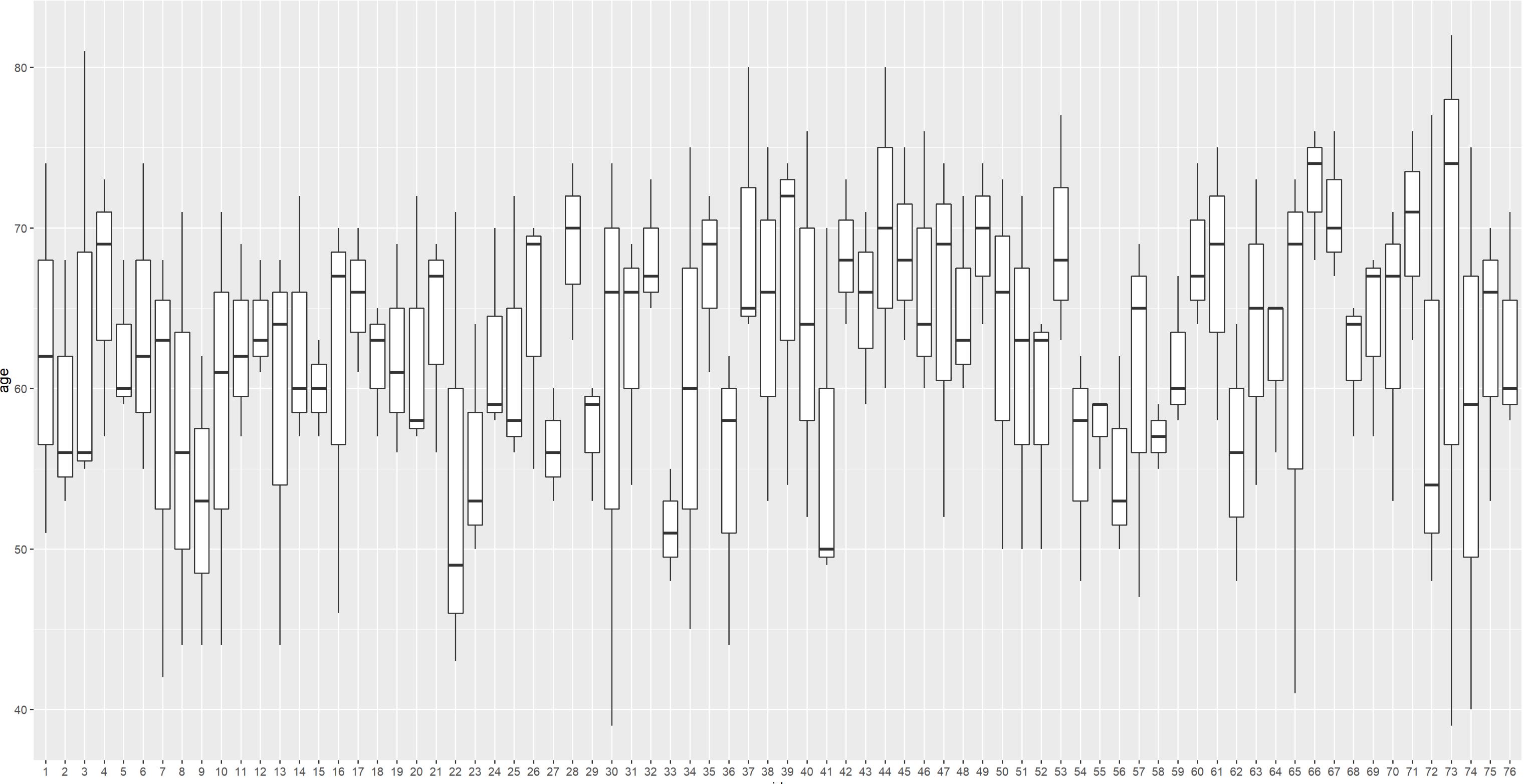
1、这里得出两个差异较大的结论,原因是我的配对分组比较随意。画出每个组的年龄分布的箱线图,可以看到差异非常大,理想的情况是比较窄的箱线。
2、所以如果数据本身基线水平比较整齐时,两种方式的差异可能不大,但如果两种基线特征差异比较大,且你在比较两组配对数据时没有考虑到这种统计学方法,会倾向生成更”大”OR值,也就是更向两端的值,在本文就是OR值更小(0.486<0.617)。
3、SPSS和R中计算的不一样,可能是似然比计算上细微的差距
library(ggplot2)
data_lung$id<-factor(data_lung$id)   #id需要转化为因子
ggplot(data = data_lung,mapping = aes(x = id, y = age))+
  geom_boxplot()